GRAPH OBJECTS
Overview
A graph is an object that can be placed on to the design. The purpose of a graph is to control a particular simulation and display the results of that simulation. The type of analysis performed by the simulation is determined by the type of the graph placed. The part of the design that is simulated and the data that is displayed on the graph is determined by the probe and generator objects that have been added to the graph.
The Current Graph
All graph-specific commands are on the Graph menu. The lower portion of this menu also contains a list of all the graphs in the design, with the current graph being marked by a small marker at the left of its name. The current graph is the last graph that was simulated or acted upon by a command.
Any command from the Graph menu can be invoked for a specific graph by pointing at the graph with the mouse and using the command's keyboard short-cut (shown on the menu to the right of the command). If the mouse pointer is not pointing at a graph, or if you select the command directly from the menu, the command is invoked for the current graph.
Placing Graphs
To place a graph:
- Select the graph icon.
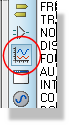
- Select the type of graph you wish to place from the Object Selector.
- Place the mouse in the Editing Window and left click at the point you wish the top left corner of the graph to appear. Move the mouse to expand a rectangle of the size of the graph you want to place and then left click the mouse again to commit the placement.
Editing Graphs
All graphs can be moved, resized or edited to change their properties using the standard schematic editing techniques.
The properties of a graph are changed on its edit dialogue form, which is opened either by first tagging the graph and then clicking the left mouse button on it, or by pointing at the graph and selecting the Edit Graph... command on the Graph menu. The form is titled for the analysis type, so an analogue transient graph opens the Edit Transient Graph form.
As well as the analysis parameters, this form carries the options that govern how the run is carried out, among them Always simulate:, Live Updates and Log netlist(s):. These are described in What Happens When You Press the Space-Bar and Live Updates.
Adding Traces To A Graph
Each graph displays one or more traces. Each trace normally displays the data associated with a single generator or probe. However, for analogue and mixed graph types it is possible to set up a single trace to display the data from between one and four probes combined by a mathematical formula which we call a trace expression.
Each trace has a label that is displayed alongside the y-axis to which the trace is assigned. Some graph types have only one y-axis and there is no option to assign the trace to a particular y-axis. By default, the name of a new trace is the same as the name of the probe (or the first probe in the trace's expression); this can be changed by editing the trace.
Traces can be defined in one of three ways:
- Dragging and dropping an individual generator or probe on to the relevant graph.
- Tagging a selection of probes and using the Quick Add feature of the Add Traces... command.
- Using the Add Traces... command's dialogue form.
The first two methods are quick to use but limit you to adding a new trace for each generator or probe assigned to the graph. The third method is somewhat more involved but gives greater control over the type of trace added to the graph. In particular, traces that require trace expressions must be added to the graph via the Add Traces dialogue form.
To drag-and-drop a probe or generator on to a graph:
- Tag the generator or probe you wish to add to a graph by left clicking on it.
- With the mouse over the generator/probe (the cursor should change to an orthogonally pointing arrow) depress the left mouse button on the generator or probe, drag over to the graph and release the mouse button.
A new trace is created and added to the graph; the new trace displays the data associated with the individual probe/generator. Note that any existing traces may be shrunk in order to accommodate the new trace.
For graphs with two y-axes, releasing the probe or generator on the left or right half of the graph assigns the new trace to the respective axis. On a mixed analogue and digital transient graph the trace type follows where you drop: release the probe or generator over the digital band at the foot of the graph and you get a digital trace, release it above that band and you get an analogue trace.
To quick-add several generators or probes to a graph:
- Ensure the graph you wish to add the generators or probes to is the current graph. The current graph is the graph whose title is shown selected on the Graph menu.
- Tag each generator or probe you want to add to the graph.
- Select the Add Traces... command on the Graph menu, or press CTRL+T. As a result of the tagged probes and generators, the command first displays a Quick add tagged probes? prompt.
- Select the Yes button to add the tagged generators and probes to the current graph.
A new trace is created for each tagged generator or probe and is added to the graph in alphabetical order; each new trace displays the data associated with its associated individual generator or probe. Traces are always assigned to the left y-axis for graph types that support two axes.
The Add Trace Command Dialogue Form
Assuming you are not performing Quick Add, the Add Traces... command displays a dialogue form titled for the analysis type, so a transient graph opens ADD TRANSIENT TRACE and a frequency graph opens ADD PHASOR TRACE. The form allows you to select the name of the new trace, its type, the axis to which it is to be added, up to four generators or probes whose data it is to use, and an expression that combines the data of the selected generators and probes.
Four trace types are offered in the Trace Type: group: Analog, Digital, Phasor and Noise. Only those trace types applicable to the graph are enabled: a frequency, AC sweep or distortion graph uses phasor traces, and a noise graph uses noise traces.
The Axis: group offers Left, Right and Reference. Left and Right assign the trace to the respective y-axis and are the only two options available to an analogue or noise trace; the whole group is unavailable for a digital trace. Reference is available only for a phasor trace, that is on a frequency, AC sweep or distortion graph, and it does not create a trace at all: the generator you select becomes the graph's reference generator, the swept source against which the other traces are measured. Only an analogue generator can be used in this way.
To add a trace to a graph using the Add Traces command
- Invoke the Add
Traces... command on the Graph
menu against the graph to which you want to add a new trace.
If there are any tagged probes or generators, a Quick add tagged probes? prompt will be presented. Respond by selecting the No button. - Select the type of trace you wish to add to the graph by selecting the appropriate Trace Type button. Only those trace types applicable to the graph are enabled.
- Select the axis to which the new trace is to be added. Only those axes applicable to the graph and trace type selected are enabled.
- Choose a probe or generator from each of the
Probe P1: to Probe
P4: dropdown lists, as many as your expression needs. Select
<NONE>
to clear one again.
If the trace type does not support a trace expression, only Probe P1: is enabled and the new trace displays the data associated with that probe alone. - Check the trace expression in the
Expression: field. Proteus
composes it for you as the sum of the probes you have selected, so
choosing three probes gives you
P1+P2+P3,
and you can then edit it into the formula you actually want. Within
the expression the selected probes are represented by the names P1,
P2, P3 and P4, matching the dropdown each was chosen from. An expression
can be up to 50 characters long.
For a trace type that does not support an expression the field is fixed at P1 and cannot be edited. - Select the OK button to add the new trace to the graph.
On a mixed graph the Trace Type selection defaults to Analog while the graph has no digital traces, and to Digital once it has one.
Editing Graph Traces
An individual trace on a graph can be edited to change its name or expression.
To tag, edit and untag a graph trace:
- Ensure the graph displaying the trace to be edited is not tagged.
- Tag the trace by clicking the right mouse button on the trace's name. A tagged trace displays its name highlighted.
- Click the left mouse button on the trace's name. The trace displays its Edit Graph Trace dialogue form.
- Edit the trace's name or expression as required. For a trace type that does not support trace expressions the Expression: field cannot be edited.
- Select the OK button to accept the changes.
- Untag the trace by clicking the right mouse button over the graph, but not over any trace names.
The Edit Graph Trace form also carries a Show data points? option, which marks the individual simulated data points along the trace. See Edit Graph Trace for a description of each field on the form.
Right clicking on a trace also brings up a context menu carrying three commands: Drag Trace Label, which starts a drag of the label to change the trace order and colour, Edit Trace Properties, which opens the Edit Graph Trace form, and Delete Trace, which removes the trace from the graph.
Changing the Order and/or Colour of Graph Traces
The order of the traces on a graph can be adjusted by dragging the labels with the left mouse button. The trace can be tagged or otherwise, as you wish.
- For digital traces the purpose of moving them is simply that of obtaining a particular stacking sequence on the graph.
- For an analogue graph, you can both drag the traces from the left to right axis and back. You can also change the colour assignments, which are made on the basis of the stack order, by shuffling the vertical stacking order.
The colours assigned to the sequence positions can be reconfigured with the Set Graph & Trace Colours command on the Template menu, or with the same command on the Options menu of a graph window. There is no need to open a graph in its own window first if you use the Template menu route.
Manual Y-Axis Configuration
By default the Y-Axes of a graph are auto scaled to provide maximum visibility for the traces on the graph. In some situations, typically where you may want to compare two or more graphs on the schematic, this effect is not desirable. In these situations Proteus provides a mechanism to set and lock both the left and right Y-axis of appropriate graph types.
To manually specify Y-axis ranges
- Place the graph, add the traces as normal and simulate the graph.
After the first simulation run the Y-axis of the graph will auto-scale. Right click on the graph object and then left click to edit. The graph's edit dialogue will appear with a Set Y-Scales option at the bottom left.
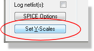
- Click on this option to get the Set Y-Axis Scaling
dialogue.
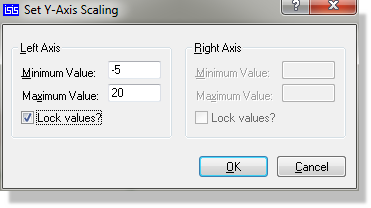
Click the Lock Values checkbox on the appropriate axis and enter the minimum and maximum values as required.
Each axis is configurable only when it has traces with a usable range, so the controls for an axis the graph does not use are unavailable, and both halves are unavailable until the graph has been simulated at least once. A lock is cleared again if its axis later loses all its traces. If you enter a minimum above the maximum, the value is rejected when you select OK, with a message such as "Left axis minimum value is greater than maximum value."- Close the dialogue and re-simulate.
See Also: